Mythical Lucca Labyrinths

On February 12, 2021 By doug14226In Programming, Travel1 Comment

Labyrinth carved on a pillar of the portico of Lucca Cathedral, Tuscany, Italy. The Latin inscription says “HIC QUEM CRETICUS EDIT. DAEDALUS EST LABERINTHUS . DE QUO NULLUS VADERE . QUIVIT QUI FUIT INTUS . NI THESEUS GRATIS ADRIANE . STAMINE JUTUS”, i.e. “This is the labyrinth built by Dedalus of Crete; all who entered therein were lost, save Theseus, thanks to Ariadne’s thread.”
Photos and quote by: Myrabella / Wikimedia Commons, CC BY-SA 3.0

For years I thought of labyrinths as simple objects. If one followed the path, the designer presented no choices. Eventually, one would exit or die in the mouth of a monster. The outcome was not your choice but the intention of the designer of the labyrinth.

Then in the fall of 2018, my attitude changed. While visiting Lucca, I had a wild thought. I would create mythical labyrinths of Lucca. They would be of the same species but different individuals.

What is the genome of the Lucca labyrinth? I had no idea. How would I design mythical descendants? Again, I had no idea. However, I did know how to start the design of a computer program. First, I needed a vocabulary to describe the program. Graph theory, a branch of mathematics that describes things (called vertices or nodes) and their relationships (called edges or links), provided that vocabulary. The following figure is a simple graph.

Figure By::AzaToth , Public Domain, Commons Wikimedia

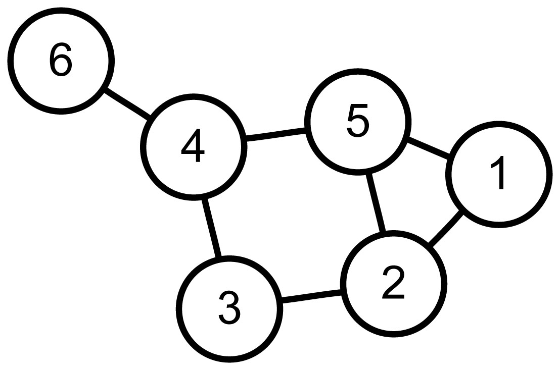
If node one is a labyrinth entrance and node six the exit. Then "walking" 1-5-4-6 is one of many paths. However, for my mythical labyrinths, I need a Hamilton path. Hamilton paths are the result of self-avoiding walks that visit all nodes. For this graph, 1-5-2-3-4-6 is a Hamilton path.

My design uses a graph that maps each location (the nodes) to neighboring nodes (using edges). The program then iterates randomly over Hamilton paths through the nodes. It halts when it finds a mythical Lucca labyrinth.

I plan two more posts about this work.

The next will describe the method of iterating over possible paths.
The final post will describe the halting condition. That is the definition of mythical Lucca labyrinths.

The remainder of this post addresses the graph design and its relationship with the drawing of the labyrinth.

Returning from Lucca, I printed an drawing of the labyrinth. Taking a red magic marker, I attempted to discover the form of a graph and its path, which could describe both the Lucca labyrinth and its mythical siblings. The first and unmistakable set of nodes follows.

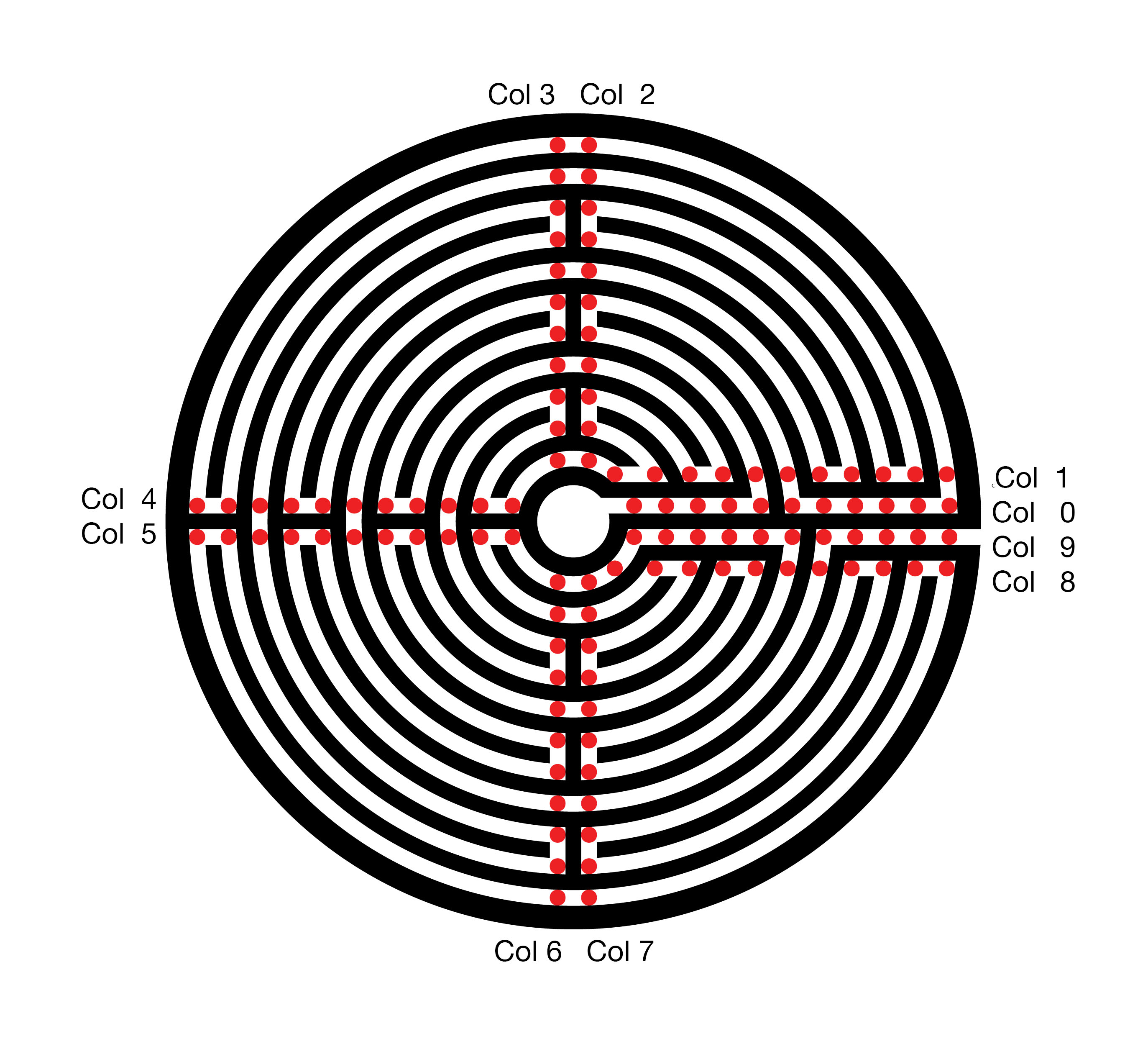
The resultant graph and path, in red, follow.

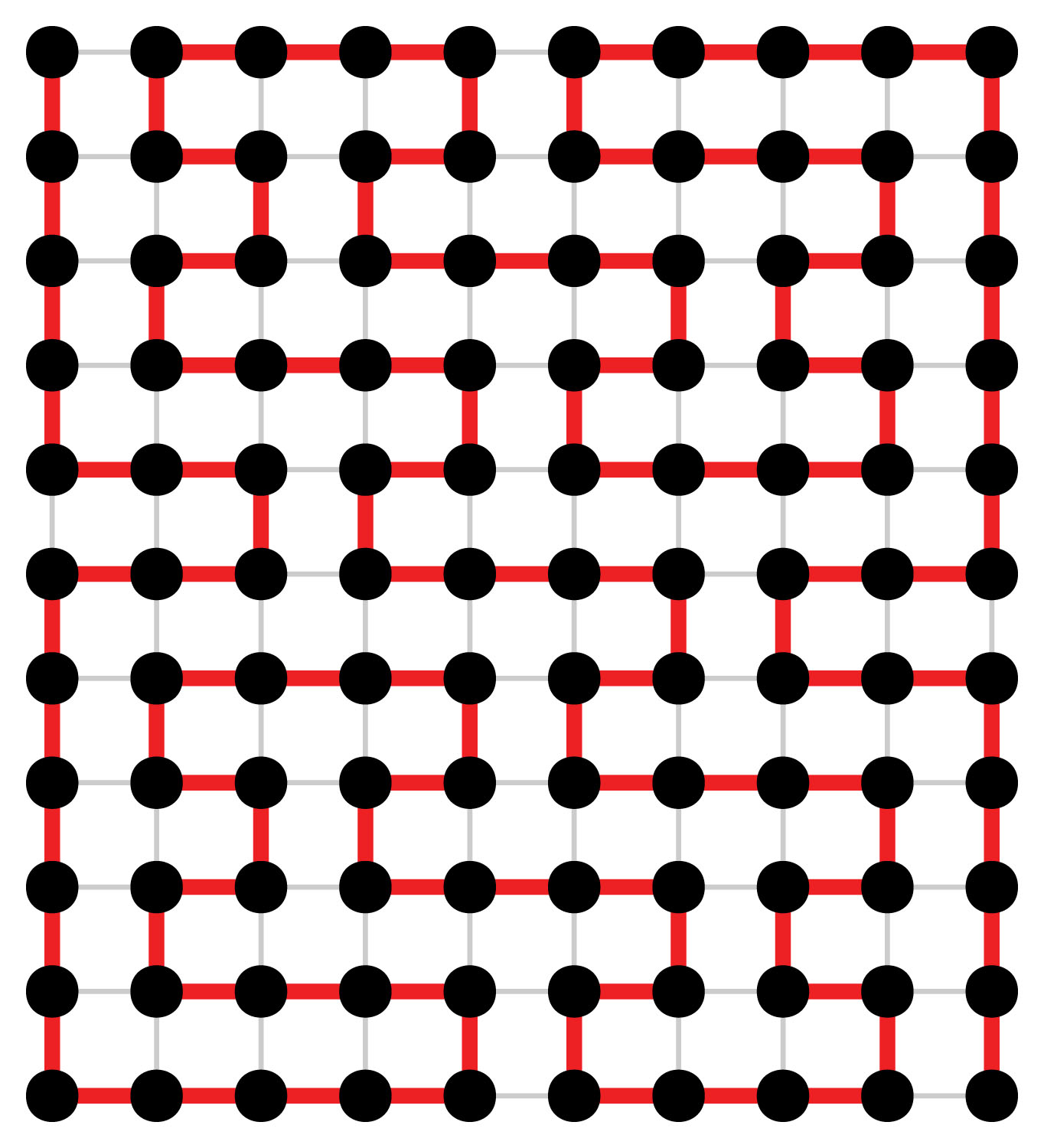
The top row of the graph, row 0, describes the central ring of the labyrinth. The bottom row, 10, maps the outer ring of the labyrinth. The exit from the labyrinth’s central court, column 0, is to the left and the path to the exterior is to the right. The red Hamilton path describes the route of the labyrinth.

This eleven by ten rectangular graph might satisfy my needs. However, it has a fatal flaw. In every row, the path connects the odd columns 1, 3, … 11 to the even column to their right. My mythical labyrinths will also require these connections. Without all of these connections, some of the sweeping arcs will be missing. These arcs are a chief feature of the Lucca labyrinth and, therefore, also required for my myths. Using this Graph, the search space for my mythical labyrinths is very substantial. The program run time will be significantly increased, probably beyond my lifespan and that of my computer.

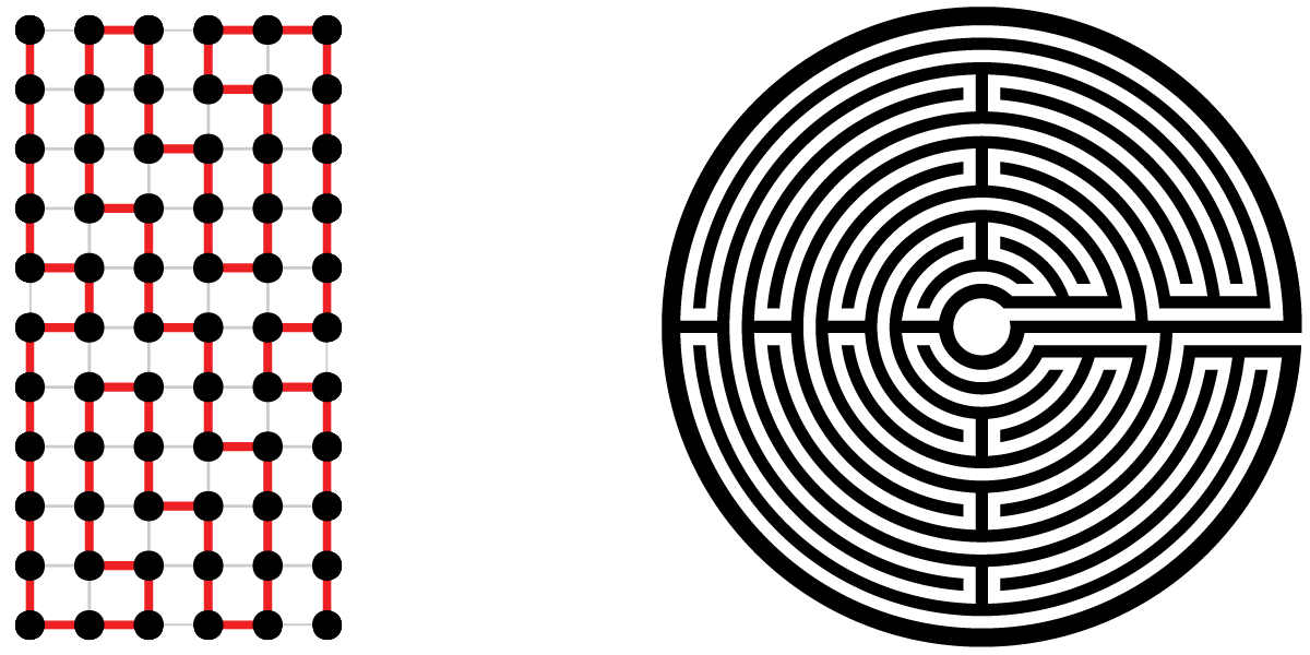
Replacing each pair of nodes, which will always be connected, with a single node avoids checking 44 edges to ensure their presence. However, the new graph does not contain information on every turn. The labyrinth drawing software must cover this missing information. The following analogy illustrates my design. Think of the labyrinth interior columns as a snowboarder performing on four connected half-pipes. When our snowboarder enters the half-pipe, gravity and then inertia takes him with no alternatives to the opposite edge. Then if directed to the next column, the snowboarder exits the half-pipe. When remaining in the half-pipe, the snowboarder first turns 180 to the next row. Then once again, gravity and inertia drive our snowboarder back across the half-pipe.

The eleven by six graph and drawing for the Lucca labyrinth follow.

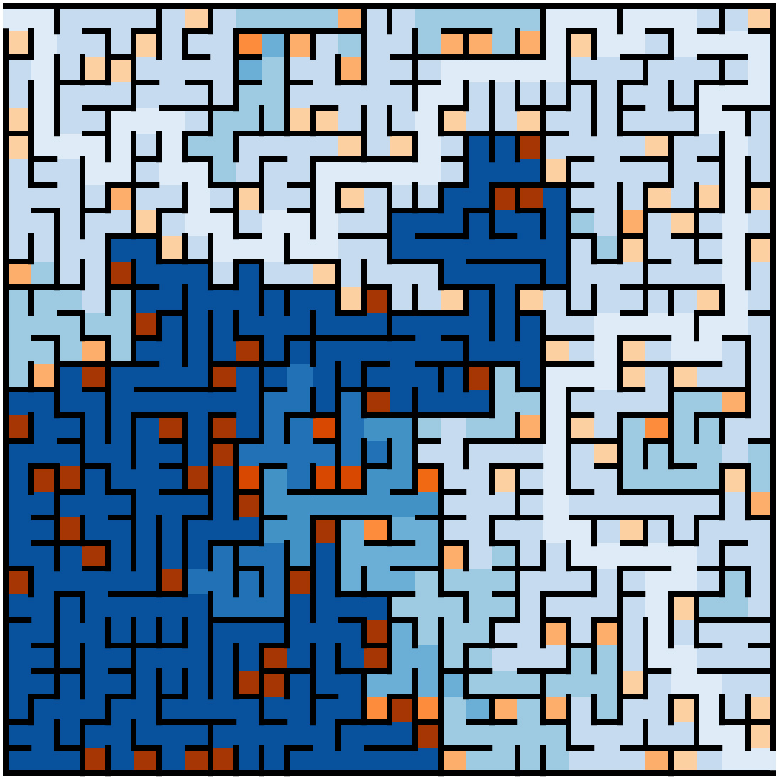
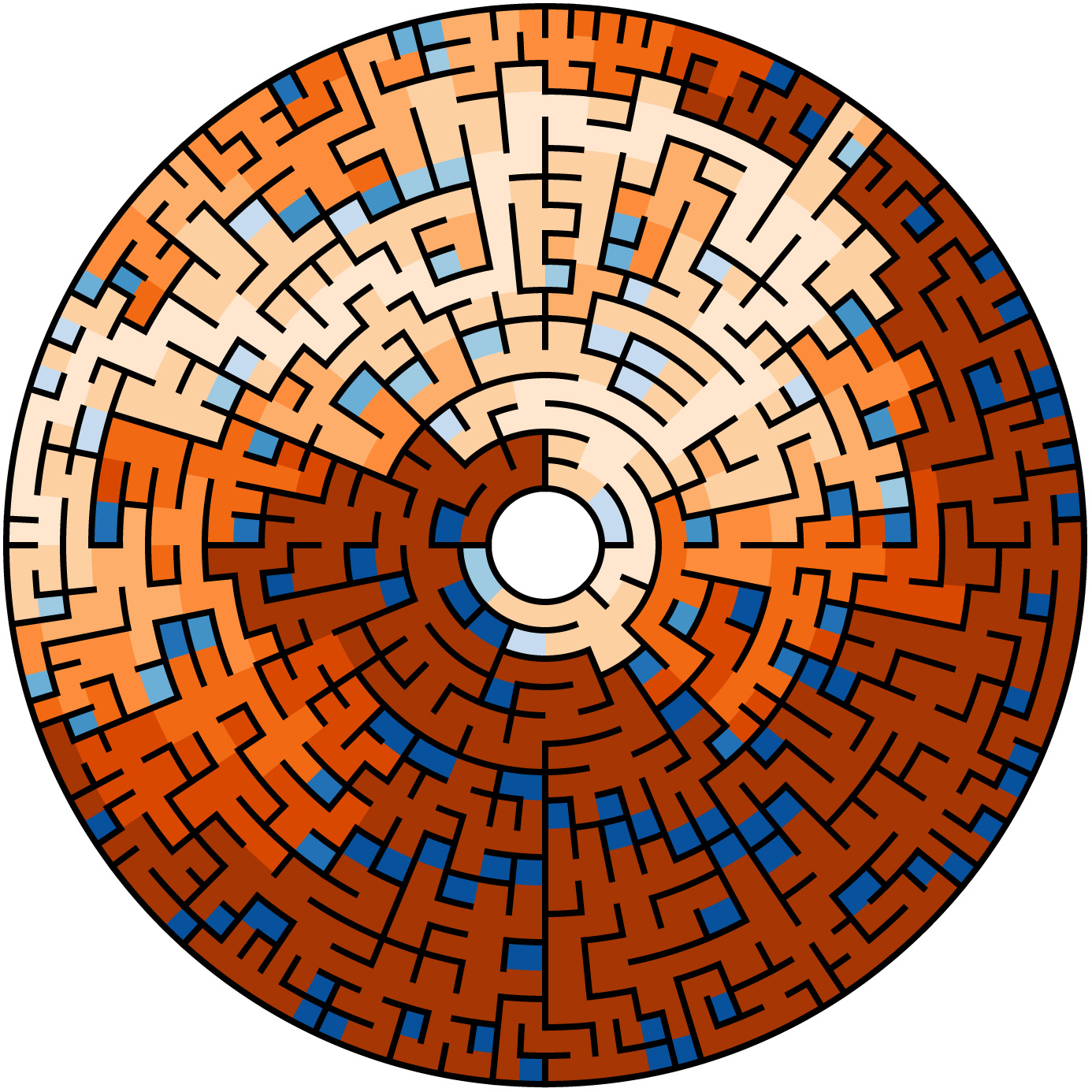
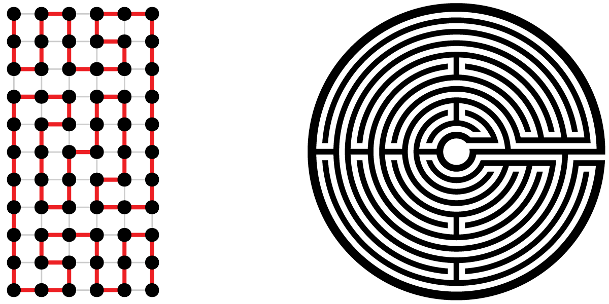
In closing, here are two of my mythical Lucca labyrinths.

Predicting Football Playoff Scores

On February 2, 2019February 2, 2019 By doug14226In Programming1 Comment

For or the last month I have been struggling to publish a ~~credible~~ machine learning prediction of NFL playoff scores. Why? Because I want to get my hands dirty with data analytics. Why football? Because politics and or social issues might lose friends, financial markets might lose friends’ money, and science stuff would be just too dry. Besides most of my friends have some interest in football.

Two weeks ago I published my predictions for the AFC and NFC Championship Games. Since that time I have been transferring my code to Google Colaboratory, so you can run it, and writing this blog post. Now it is the eve of Super Bowl LIII and time to wrap it up. My prediction? LA 29 NE 23. Would I bet on it? No way.

At this point in the post, I suggest you run my code and see all of this year’s playoff score predictions. Click on “Open in Colab” below. Using the “Runtime” menu, select “Run all.” Then scroll the right pane to the bottom and wait for the scores to compute.

Am I pleased with my program? Yes, I set out to learn new skills, mission accomplished. Is it accurate? Sometimes. You will note that have I nailed both LA scores and missed badly on the low side with New England. I obviously have work to do.

I plan to continue improving the program over the next year. The effort to date has been a freewheeling hacker approach. I need to introduce “light” engineering formalism. Starting with testing after each change using past seasons. Something like, admit changes only it improves in three out of four seasons.

For those of you who have no interest in the details, this is a good point to leave. I will post on this blog each time I learn major new concepts about machine learning or football,

The first step is always, where to get data? Was this project going to end before it started? Luckily for NFL football game data, someone else has done most of the work. Andrew Gallant’s (aka Burntsushi) NFLDB provides an interface from NFL game day on the web to a PostgreSQL database on my MacBook Pro. The only downside to NFLDB is that it uses Python 2.7 and I am committed to Python 3. So now I have Python 2.7 with the Burntsushi software, but this is not a great inconvenience since I only use it to update a PostgreSQL database. Also, I added psycopg2, as an interface to PostgreSQL, to my Python 3.

What is the data provided through NFLDB? A hierarchical set of data tables. The highest level is “game.” It contains the teams, who’s home, the final and quarter scores. The second level is “drive.” Its contents include the drive start (time and yard-line), the end condition, e.g. (Touchdown, Field Goal, Punt, Interception, Fumble, etc.) along with the yard line, the number of first downs, yards gained, penalty yards and elapsed time. The drive data is the end of the data which I have used for this first version of my algorithm. Below the drive, there is “play,” “play-player” and “player” data. These tables are detailed at a sufficient level to call the game for a radio broadcast. Who carried the ball, threw the pass, to which intended receiver, and on the defense, who made the tackle, and who assisted? With NFLDB the answers to all of these questions are yours.

How does one predict a result (e.g. a Football score) from data? Three different components must be chosen. A mathematical model for the result needs to be selected. This model can range from a linear equation to a many layer neural network. Secondly one develops a list of features which are chosen from or calculated from the data. Finally, a training algorithm or process is chosen. Another expression for the training algorithm is machine learning.

I am using is a simple linear equation to model football scores.

$Score_o= \omega_h * Home + \sum_{n=1}^{k_p}\omega_n*O_n + \sum_{m=1}^{k_d}\omega_m*D_m$

Where $Score_o$ is the score fitted/predicted for the team, $Home$ is one if the team is home zero otherwise, $O_n$ are offensive features of the team, and $D_m$ are the defensive features of the opposing team. Finally, the $\omega$ s are the weights fitted by the training algorithm.

Useful features are correlated with the football scores. Also, they need to be much smaller in number than the data they will be fitted to. The football regular season has 256 games yielding 512 team scores. If we choose 512 features our fit to the model will only describe what has happened and have no predictive power. I picked my feature set primarily as a set of probability estimates. The table below describes the offensive features. To be more correct, read probability as the probability estimate from the regular season. I have also incorporated the possibility of measurement per play features, and have added one example “pyp” which is net penalty yards per play.

Turnover	Probability that an offensive drive results in a turnover.
safety	Probability that an offensive drive results in a safety.
TDle20	Probability that an offensive drive, starting between own goalline and own 20, results in a Touchdown.
TDle40	Probability that an offensive drive, starting between own 20 and own 40, results in a Touchdown.
TDle60	Probability that an offensive drive, starting between own 40 and opposing 40. results in a Touchdown.
TDle80	Probability that an offensive drive, starting between opposing 40 and opposing 20. results in a Touchdown.
FGle20	Probability that an offensive drive, starting between own goal-line and own 20, results in a Field Goal.
FGle40	Probability that an offensive drive, starting between own 20 and own 40, results in a Field Goal.
FGle60	Probability that an offensive drive, starting between own 40 and opposing 40, results in a Field Goal.
FGle80	Probability that an offensive drive, starting between opposing 40 and opposing 20, results in a Field Goal.
RZ	Probability that an offensive drive which reaches the opposing 20 results in a Touchdown.
nfd	Probability that an offensive drive, with no first downs, results in a Punt.
Ple20	Probability that an offensive drive starts between own goal-line and own 20.
Ple40	Probability that an offensive drive starts between own 20 and own 40.
Ple60	Probability that an offensive drive starts between own 40 and opposing 40.
Ple80	Probability that an offensive drive starts between opposing 40 and opposing 20.
pyp	Average yards lost per play as a result of a penalty.

What about defense? I have used the same measures as the offensive measures. Instead of the offensive team against all competitors, I calculated each parameter for all competitors against the defensive team. Yes, the direction of goodness is reversed, but the model can handle that. For example, a good defense will have a lower probability of allowing a touchdown in the Red Zone. These new parameters use the same name with a preceding “D.”

To train my model, I use Bayesian Ridge Regression from Scikit-Learn. Why? Because I read somewhere, it minimizes the problems with multicolinearity and overfitting with inappropriate features.

If you have not run the code yet, I suggest you click on “Open in Colab” below:

I changed my approach to initialization of the enviornment from my previous Colaboratory notebooks. This time i used %%Shell to write a shall script to load the data files. On my own Mac I used SQL for my Pandas dataframes. Saving off to “csv” files seems to be a good way to move to Colabortory.

First maze notebook

On December 11, 2018February 2, 2019 By doug14226In Programming1 Comment

My love of programming mazes started with the purchase of “Mazes for Programmers: code your own twisty little passages,” see A-mazing books. For almost two years I have often returned to mazes, programming just for fun.

This Colaboratory notebook cuts maze programming to its basics. To build the notebook, I have taken my current python maze packages and removed all code except for that required for this project. By minimizing the code, I can show it all in the notebook; I have no hidden tricks. My goal was to produce a maze puzzle, a perfect maze with only one solution.

To open this notebook click the following icon:

The easiest way to run the maze program is to select “Run all” from the “Runtime” menu. The program will generate and print to PDF a maze of the size specified on the Maze Parameters form. To download this PDF check the “downloadPDF” box on the “Output” form and select “Run the focused cell.”

For more detail Continue.

For an overview of my colabortory python notebooks take a look at Non Photo-Realistic Mona Lisa, Revisited. This previous post introduces the manner in which I have structured my notebooks, for this maze notebook, I have used a similar structure.

Regarding copyrights and license, The maze generation code originated in the Ruby programming language in the book “Mazes for Programmers: code your own twisty little passages” by Jamis Buck. Sami Salkosuo translated these into Python. I have added a new concept to the Distances class, that is distance off the solution path. Adapted the cell class to more directly support other cell shapes such as polar, hex, and 3D. Finally, I added the Cairo drawing routines to both the Cell and Grid classes.

Section 1: is a direct lift from Non Photo-Realistic Mona Lisa, Revisited. to install the Cairo drawing package

Section 2 defines the Cell class. The class describes the data and methods implementing each cell of the maze. This data includes the cell’s neighbors and which of the neighbors are connected by missing walls. When drawing the maze, fillCell is used to color the background, and drawCell constructs the walls. Note, since the maze is drawn top to bottom, west to east, only the east and south walls are considered by drawCell.

Section 3 defines the Distances class. Jamis Buck and Sami Salkosuo both defined distances as the distance from a cell to all other cells. I added defininitions for add and sub so that algebraic combinations such as distance from the solution path are possible.

Section 4 defines the Grid class including the data and methods for implementing each maze. My main additions are getDistancesFromPath which uses distance algebra to define distance off the path as the distance from start + distance from goal – path length, and the drawing routine drawGrid and draw Opening. Unlike other maze programs I have written this one produces a PDF document. First, it illustrates the unsolved maze and then on a second page provides the solution. Most of the drawing code is directly from my work with scalable vector graphics. To produce page filling pdf files, I used the Cairo scale and translate functions. These provided the transformation from my arbitrary SVG space to the fixed paper mapping of PDF.

Section 5 implements the Wilson algorithm for maze generation. For Jamis Buck’s description of this algorithm and his original Ruby code follow this link.

Finally the main routine imports the required python packages, reads the user input from a form, Generates a “Grid,” initializes it with “initWilsonMaze,” chooses random entry and exit columns with ” randint” and produces the PDF file with “drawGrid.” displayMaze reads the binary png image from the Cairo surface and displays it in the notebook.

The last two cells are provided to download the pdf to your computer and to download setup.log if problems occur.

If you haven’t launched the app yet, click the icon.

Non Photo-Realistic Mona Lisa, Revisited

On December 6, 2018February 2, 2019 By doug14226In Programming1 Comment

Since I last wrote on stippling or half-toning algorithms in Non Photo-Realistic Mona Lisa, I have developed a new image tiling algorithm and finalized my plans and procedures for sharing python code.

Algorithm Update

My original algorithm divided the input photo into n equal black rectangles by slicing in one direction, then each of these rectangles was divided, … Although this method produced very recognizable results, it also produced patterns which were artifacts of the algorithm in the image.

The two images below illustrate the first slice into 5 rectangles of equal blackness, followed by a second slicing of each of the 5 into 5 more using the original algorithm.

In an attempt to break up the artifact patterns, I have developed a new approach which uses recursion to slice up rectangles. Instead of selecting n slices of equal black ink the new code first looks for the most significant slice it can remove containing 1/N’th of the ink from either end and then recursively calls itself to process N-1 slices which may now switch directions.

The figures above illustrate the approach for division by 5 followed by a second division by 5. First, the algorithm finds the most massive horizontal fifth at the top end of the verticle image. Next, one-fourth of the left side of the remainder is chosen. Then the top third of the rest is selected, and then the final portion is split into left and right. In the second pass, illustrated by the image on the right, each of these rectangles is processed similarly. Note that the rectangles appear more random than those generated by the original algorithm.

What are these algorithms for. First for some images the output rectangles have an incredible abstract beauty of their own. My future plans include both geometric pattern half-tone images, were an icon of the correct size represents the actual black content, and photo mosaics where a small photo is placed in the center of each rectangle and when viewed from a distance they merge into the original image.

Run The Code

The big news is, I have finalized the procedures I will use to share the code I write. Google’s Colabortory provides a Linux processor on which you can execute Python Jupyter Notebooks. The easiest way would have been to store my Notebooks on a Google Drive and share them granting permission to view and comment to all. However, the process of transferring ownership of a copy so that it can be executed and/or changed without modifying the original seemed overly complicated. In the end, I decided to use Github.com for my storage of Notebooks. Colabortory provides tools which open my Github repository Notebooks as copies owned by you, Oh, you will need a Google account. If you’re not currently logged in, colaboratory provides a button to start the log in process.

Colabortory provides menus and buttons in the toolbar at the top of the page. Of specific interest now are the file menu which will allow you to save the Notebook (file type .ipnb) on your Google drive, in Github, or download to your computer, and the run menu in which the run all command can be used to execute the notebook.

At this point I suggest you open the Photo_SlicerTiler notebook. Click on the Icon below to open the Notebook in a new Tab or Window (depending on your browser settings).

Under the Notebook toolbar, you will find two window panes. To the left is a Table of contents which allows navigation through the notebook and to the right the notebook code. The right pane is divided into cells which contain either text (Markdown formatted) or code. The runtime menu controls the execution of the notebook. Code cells can all be executed one after the other with “Run all,” or a few cells can be run with “Run Selected” or they can be “single stepped” with “Run the focused cell.”

The code cell of the first section “Setup Python environment” first checks for the existence of the Cairo drawing package and the Mona_Lisa.jpg file. If both exist, it exits. This avoids the setup overhead for multiple executions with changing parameters. The Setup also produces a Log to aid in locating problems.

Three Linux commands are used in the setup. Note the “!” is used to execute the Linux command from the python environment. When the “!” is used the output of the Linux command is returned as a string to python.

“apt-get” is part of the Debian/Ubuntu Linux package management system and is used to install libcairo2-dev the Cairo library.

“pip3” is the python3 package manager and is used to install pycairo the python interface to the binary library.

And finally “wget” is used to download Mona_Lisa.jpg from the drive.google.com using https. The sharable link to Mona_Lisa.jpg on my Google drive is https://drive.google.com/open?id=1_hUkSmQjXfxMwq170pOlRxdgf7hajgHd

The portion of this link following “id=” is the Google fileID. These fileIDs can be used in wget commands to download to your Colaboratory environment. The required form is:

wget -O ColabFileName “https://drive.google.com/uc?export=download&id=FileID“

The capability to run sharable notebooks from Github and the capacity to access data from a google drive with wget are two pillars of secure runnable shared code on Colaboratory.

Sections 2 and 3 are “libraries”. Section two defines the sliceIm and tileIm functions which implement the algorithms described at the top of this post. drawImage a function defined in section three creates a scalable vector graphics drawing of the rectangles produced by sliceIm or tileIm.

A great advantage of Cairo when used within Colaboratory/Jupyter notebooks is that regardless of the graphics backend used (SVG, PDF, JPEG, Microsoft-Windows …), one can always produce a PNG image file by calling cairo.Surface method write_to_png. The displayImage function uses write_to_png to produce an in-memory ByteString. The IPhython.core.display Image method converts the ByteString to type png image so that the IPhython.core.display.display method can produce the drawing in the notebook output.

The first cell of section 4 (The main program) first imports the required python packages and then reads the input image. Open, from the Python Image Library (PIL), supports most computer image file formats. Convert is used to convert color photos to black and white using industry standard conversion. The last two lines of the cell use the numpy package to produce a “negative” image array with black as 1.0 and white as 0.0.

The next cell contains a new construct. It implements a notebook form. A form is a simple user interface for entering data into the program. When you change data in the form, the code changes to assign the new value.

The second portion of the cell defines a main procedure which iterates over the divisors entered and slices or tiles each rectangle by the current divisor. Why is main defined and not just scripted python? Because if it’s a script the Cairo surface will remain defined, the output file will not be closed, and the download cell below will download an empty file. When we exit main, the surface is freed, and the file is closed.

The last two cells are conditional, on the checkbox of the form, downloads of the output and setup.log.

Please post comments about this blog using the comment link. If you have issues, suggestions, improvements etc. regarding the code go to https://github.com/doug14226/colab1/issues and open a new issue.

Next code example will geenerate mazes, until then try a little programing, add code to upload your photo and change the code to use it.

We can write code together!

On October 17, 2018 By doug14226In ProgrammingLeave a comment

I am really excited about the Google internet app Colaboratory. For the first time, I can envision a community sharing computer ideas and code, without being concerned with whether they are running a Macintosh, Windows 10 or Linux machine. In fact, users of iPads, Surface Go, and Android tablets can join in on the fun.

Colabortory provides a web-based implementation of iPython/Jupyter notebooks. Since it is web-based, an extra level of safety is ensured in sharing programs. The code or its products will not be downloaded to your machine without your permission. Colabortory also implements a “playground” mode where no files are written to your computer or to your google drive.

I have plans to write and publish the following programs to be shared with all:

Mazes, a maze generation “system” for fun, art or storytelling.
Football, machine learning to predict the Super Bowl winner
Fantasy Football, machine learning to improve your fantasy team draft
Image Processing — new “filters” for your photos
Social Barometer — machine learning interpretation of Twitter posts from fans of your local sports team.
If you have other computer program suggestions, please forward them in your comments. To participate in this experiment, you will need a google account with google drive. It’s free to set up that account and join in the fun. drive.google.com
Finally, I promise to provide means for users to inspect all of my source code. Also, I will never offer programs without source, such as byte compiled python .pyc or C executables. I do not want a stranger’s compiled code and neither should you.

A-mazing books

On October 3, 2018October 4, 2018 By doug14226In Programming, Reading3 Comments

One of the tricks I commonly use when visiting a bookstore is to force myself to buy only one book. It can’t be the book reviewed last weekend in the New York Times, nor can it be a book I always intended read, it has to be unusual, unlike any of my past reading.

I use this trick while in Seattle, January 2017. We had just watched the Chinese New Year street parade, with long dragons dancing down the street, followed by acrobats and dancers. With my mind charged with the exotic, I entered the downtown Barnes& Noble store where I preceded to shop. It’s common with me when picking just one book to select a translation of a foreign novel or a new edition of poetry by a poet I have never read. However, my one book has never addressed computer programming. But, when I saw “Mazes for Programmers: code your own twisty little passages” and read the back cover comments, “A book on mazes? Seriously? Yes! Because it’s fun. Remember when programming used to be fun?”, I was hooked.

Over the next several weeks I read the book cover to cover trying to understand all of the examples. One problem I had is, the author of the book had written all example code in Ruby, a language which I have never used. I had selected Python as my one language of choice to use for retirement hobby computing. The difference between two computer languages, even though they are in some ways similar, as Ruby and Python are both object-oriented languages, is complex. It’s like the computer translation of human communication. For an example of this difficulty, I took the first sentence above and translated it from English to Italian to Hungarian and back to English with Google translate, this is the result: “One of the trick I buy in a bookstore is to force myself to choose only one book”

The problem of languages was solved when I discovered Sami Salkosuo’s posting of mayzepy on GitHub. Someone else had done the hard part for me. My work would now be concentrated on the creation of different maze types and the rendering of those mazes as computer drawings.

Almost immediately, as I started to render mazes, I realized that eventually, my software drawings would need to reference the past. I needed to understand the stories of ancient mazes in Eygpt, the Greek myth of the Minotaur, and the meditative wall and pavement mazes of the medieval church. Luckily the Buffalo library had a copy of “Mazes and Labyrinths: Their History and Development,” by W. H. Matthews. I checked it out, and as I read it, I knew I wanted a copy for reference. At this point, I discovered Amazon had a kindle version for $2.99.

Another direction of study when constructing mazes is the mathematics field of Graph Theory. A “Perfect Maze,” one without loops, is a “Connected Tree” in graph theory. The text I have been studying is “Pearls in Graph Theory” by Hartsfield and Ringel. I recommend it.

Finally here are examples of my computer generated mazes.

saved7 polar yellowHorizon2

Non Photo-Realistic Mona Lisa

On August 23, 2018September 3, 2018 By doug14226In Programming1 Comment

Over the last two years, I have been writing computer applications in Python as a hobby. During this period the possibility of using Python for image processing has been in the back of my mind. At first, Python, since it is interpreted, seemed a totally inappropriate language. Then I started using the NumPy library. NumPy provides Python a capability very similar, although very different in syntax, to the commercial software package Matlab. All I needed was an idea for my first image processing application.

A paper Modular Line-Based Halftoning via Recursive Division, provided the spark. See Proceedings of the Workshop on Non-Photorealistic Animation and Rendering, 2014 Vancouver, published by ACM New York (For a copy of the paper click on the title above and then follow a second link to get a free copy from the ACM library)

The Photo to the right is the result of my first image processing attempt. It consists totally of black rectangles. Each rectangle contains the same amount of “black ink” in the original photo. The first step sliced the photo into five rectangles of equal black ink, each of these was sliced into five more, then five more …

The final list of divisors used was 5,5,5,5,3,3,2,2,2,2, generating ninety thousand rectangles. Total execution on my old 2011 MacBook Pro is 10 seconds. Clearly, Python with NumPy is an acceptable image processing platform.

My other favorite Python concept is Cairo. Cairo is a drawing package. Think of it like an alternative PostScript. The original form of the image on the right above was Scalable Vector Graphics (SVG)
Cairo supports many “back-ends” and one of them is SVG. Click here to see a full rez of the right image.

My next version will have better imaging slicing to break up patterns. Also I plan to upload an iPython/Jupyter Notebook implementation.

Thats all for now. The next section describes a few of the coding details. If your not interested skip to the bottom and leave your comments.

Software Details

My function sliceIm, the heart of this process, follows:

def sliceIm(image, rects, n):
   nxtrects = []
   for rect in rects:
      top = rect[0]
      bottom = rect[1]
      left = rect[2]
      right = rect[3]
      im = image[top:bottom,left:right]
      if (bottom - top) > (right - left):
         rowsum = im.sum(axis=1)
         cumrowsum = rowsum.cumsum()
         xr = np.amin(cumrowsum)
         mr = (np.amax(cumrowsum)-xr)/n
         for i in range(1,n):
            t = np.amin(np.nonzero(cumrowsum>=(xr+(mr*(i-1)))))
            b = np.amin(np.nonzero(cumrowsum>=(xr+(mr*i))))
            nxtrects.append( [top + t, top + b, left, right] )
         nxtrects.append( [top + b, bottom , left, right] )
      else:
         colsum = im.sum(axis=0)
         cumcolsum = colsum.cumsum()
         xc = np.amin(cumcolsum)
         mc = (np.amax(cumcolsum)-xc)/n
         for i in range(1, n):
            r = np.amin(np.nonzero(cumcolsum>=(xc+(mc*(i-1)))))
            l = np.amin(np.nonzero(cumcolsum>=(xc+(mc*i))))
            nxtrects.append( [top, bottom, left + r, left + l] )
         nxtrects.append( [top, bottom, left + l, right] )
  return nxtrects

[notes]
image:   NumPy array of pixels (0.0 is white 1.0 is black)
rects:   lists of lists. each element is a 
         rectangle [top, bottom, left, right]
         example from second slicing of Mona Lisa:
         [[0, 269, 0, 997], [269, 537, 0, 997],
         [537, 792, 0, 997], [792, 1015, 0, 997],
         [1015, 1246, 0, 997]]
n:       number of slices to divide each rectangle
line 8:  im = image[top:bottom,left:right] 
         im is assigned a slice of image
         The slice is not copied, im is just mapped to the slice
         NumPy Magic  
line 10: rowsum = im.sum(axis=1) n by m slice summed over
         each row returning an n by 1 array
line 11: cumrowsum = rowsum.cumsum()  over slice of
         sum of all rows above
line 15: np.nonzero(cumrowsum>=(xr+(mr*(i-1)))))
         returns and n by 1 0/1 result for
         row by row comparison
         t is the min row or the t row of the new slice
line 16: finds b or the bottom of the new slice
line 20-28 repeat structure of line 10-18 for new horizontal slice

Finally here is lowest level cairo drawing routine for drawing all the rectangles.

def drawImg(rects, surface, ctx):
    for rect in rects: 
        top = rect[0]*2
        bottom = rect[1]*2
        left = rect[2]*2
        right = rect[3]*2
        ctx.rectangle(left, top, right-left, bottom-top)
        ctx.stroke()

[notes]
rects:   lists of lists. each element is a 
         rectangle 
surface: a Cairo drawing surface
ctx:     a Cairo drawing context

Doug's Paws

Category: Programming